源自於
https://www.geeksforgeeks.org/program-simpsons-13-rule/
In numerical analysis, Simpson’s 1/3 rule is a method for numerical approximation of definite integrals. Specifically, it is the following approximation:

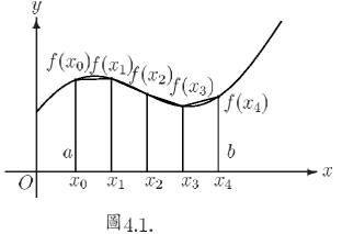
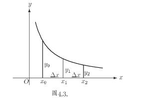
In Simpson’s 1/3 Rule, we use parabolas to approximate each part of the curve.We divide
the area into n equal segments of width Δx.
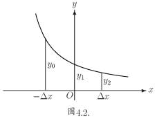
Simpson’s rule can be derived by approximating the integrand f (x) (in blue)
by the quadratic interpolant P(x) (in red).

the area into n equal segments of width Δx.
Simpson’s rule can be derived by approximating the integrand f (x) (in blue)
by the quadratic interpolant P(x) (in red).
In order to integrate any function f(x) in the interval (a, b), follow the steps given below:
1.Select a value for n, which is the number of parts the interval is divided into.
2.Calculate the width, h = (b-a)/n
3.Calculate the values of x0 to xn as x0 = a, x1 = x0 + h, …..xn-1 = xn-2 + h, xn = b.
Consider y = f(x). Now find the values of y(y0 to yn) for the corresponding x(x0 to xn) values.
4.Substitute all the above found values in the Simpson’s Rule Formula to calculate the integral value.
Approximate value of the integral can be given by Simpson’s Rule:

Note : In this rule, n must be EVEN.
Application :
It is used when it is very difficult to solve the given integral mathematically.
This rule gives approximation easily without actually knowing the integration rules.
It is used when it is very difficult to solve the given integral mathematically.
This rule gives approximation easily without actually knowing the integration rules.
Example :
Evaluate logx dx within limit 4 to 5.2.

First we will divide interval into six equal
parts as number of interval should be even.

x    :  4     4.2   4.4   4.6   4.8  5.0  5.2
logx :  1.38  1.43  1.48  1.52  1.56 1.60 1.64

Now we can calculate approximate value of integral
using above formula:
     = h/3[( 1.38 + 1.64) + 4 * (1.43 + 1.52 +
                      1.60 ) +2 *(1.48 + 1.56)]
     = 1.84
Hence the approximation of above integral is
1.827 using Simpson's 1/3 rule.
// CPP program for simpson's 1/3 rule
#include <iostream>
#include <math.h>
using namespace std;

// Function to calculate f(x)
float func(float x)
{
 return log(x);
}

// Function for approximate integral
float simpsons_(float ll, float ul, int n)
{
 // Calculating the value of h
 float h = (ul - ll) / n;

 // Array for storing value of x and f(x)
 float x[10], fx[10];

 // Calculating values of x and f(x)
 for (int i = 0; i <= n; i++) {
  x[i] = ll + i * h;
  fx[i] = func(x[i]);
 }

 // Calculating result
 float res = 0;
 for (int i = 0; i <= n; i++) {
  if (i == 0 || i == n)
   res += fx[i];
  else if (i % 2 != 0)
   res += 4 * fx[i];
  else
   res += 2 * fx[i];
 }
 res = res * (h / 3);
 return res;
}

// Driver program
int main()
{
 float lower_limit = 4; // Lower limit
 float upper_limit = 5.2; // Upper limit
 int n = 6; // Number of interval
 cout << simpsons_(lower_limit, upper_limit, n);
 return 0;
}
Output:
1.827847


Python 語言
# Python code for simpson's 1 / 3 rule
import math

# Function to calculate f(x)
def func( x ):
 return math.log(x)

# Function for approximate integral
def simpsons_( ll, ul, n ):

 # Calculating the value of h
 h = ( ul - ll )/n

 # List for storing value of x and f(x)
 x = list()
 fx = list()

 # Calcuting values of x and f(x)
 i = 0
 while i<= n:
  x.append(ll + i * h)
  fx.append(func(x[i]))
  i += 1

 # Calculating result
 res = 0
 i = 0
 while i<= n:
  if i == 0 or i == n:
   res+= fx[i]
  elif i % 2 != 0:
   res+= 4 * fx[i]
  else:
   res+= 2 * fx[i]
  i+= 1
 res = res * (h / 3)
 return res

# Driver code
lower_limit = 4 # Lower limit
upper_limit = 5.2 # Upper limit
n = 6 # Number of interval
print("%.6f"% simpsons_(lower_limit, upper_limit, n))
 。
。  。
。
 。
。
 。
。
 。
。