MIT Inventor 2 --MQTT


當設計陸上微波通信時應要考慮地球鼓起(Earth Bulge) 在圓滑的地球上(Smooth Earth) 設山頂高度為h 則無線電地平線(Radio Horizon)距離

D^2 = h^2 + 2hR 其中R=地球半徑=6,371 KM
因為 R>>h 所以D^2 = 2hR , D= (2hR) ^0.5

Let R be the radius of the Earth and h be the altitude of a telecommunication station. The line of sight distance d of this station is given by the Pythagorean theorem;
Since the altitude of the station is much less than the radius of the Earth,
If the height is given in metres, and distance in kilometres,[1]
If the height is given in feet, and the distance in statute miles,
地球半徑6,371 公里
 = 3.56959 (6371 Kilo =6.371 Mega)
* √4/3 (考慮有效地求半徑因數 k=4/3=1.333)


在點對點無線通信中,重要的是兩個無線系統之間的視線不受任何障礙物(地形、植被、建築物、風電場和許多其他障礙物)的影響。因為 LOS 中的任何干擾或障礙都可能導致信號丟失。
在安裝無線通信系統時,重要的是要保持發射天線和接收天線之間的橢圓區域沒有任何障礙物,以便系統正常運行。發射天線和接收天線之間的這個 3D 橢圓區域稱為菲涅耳區。橢圓的大小由操作頻率和兩個站點之間的距離決定。

菲涅耳區域由多個區域組成,區域 1 具有最強的信號,隨後的區域(區域 2 和區域 3)具有較弱的信號。

根據上圖,菲涅耳區使用以下公式計算。

https://www.everythingrf.com/rf-calculators/fresnel-zone-calculator
菲涅耳(發音為“Fray-nell”)區的確切理論相當複雜。然而,這個概念很容易理解:我們從惠更斯原理中知道,在波前的每個點都有新的圓形波開始,我們知道微波束在離開天線時會變寬,我們知道一個頻率的波會干擾彼此。菲涅耳區理論只是觀察從 A 到 B 的一條線,然後是該線周圍的空間,該空間有助於到達 B 點。一些波直接從 A 傳播到 B,而另一些波則沿著偏離軸的路徑傳播並到達通過反射接收器。
因此,它們的路徑更長,在直接光束和間接光束之間引入了相移。
只要相移是半波長,就會產生相消干涉:信號抵消。
採用這種方法,您會發現當反射路徑比直接路徑長不到半個波長時,反射將添加到接收信號中。相反,當反射路徑長度超過直接路徑超過一半波長時,其貢獻將降低接收功率。圖 RP 11:菲涅耳區在此鏈路上被部分遮擋,儘管視線看起來很清晰。
注意有很多可能的菲涅耳區,但我們主要關注第一個區,因為第二個區的貢獻是負的。第三區的貢獻再次是積極的,但沒有實際的方法來利用那些沒有通過第二菲涅爾區所產生的懲罰。
如果第一菲涅耳區被障礙物(例如樹木或建築物)部分阻擋,則到達遠端的信號將減弱。因此,在構建無線鏈路時,我們需要確保第一個區域沒有障礙物。在實踐中,這個區域的整個區域都沒有明確的必要性,在無線網絡中,我們的目標是清除大約 60% 的第一個菲涅耳區域的半徑。
這是計算第一個菲涅耳區半徑的一個公式:
r =
...其中 r 是以米為單位的區域半徑,d1 和 d2 是以米為單位從障礙物到鏈路端點的距離,d 是以米為單位的總鏈路距離,f 是以 MHz 為單位的頻率。
第一菲涅耳區半徑也可以直接從波長計算為:
r =
以米為單位的所有變量
很明顯,第一個菲涅耳區的最大值恰好發生在軌蹟的中間,並且可以在前面的公式中設置 d1=d2=d/2 找到它的值。請注意,公式為您提供區域的半徑,而不是地面以上的高度。
要計算離地高度,您需要從直接在兩座塔頂之間繪製的直線中減去結果。
例如,讓我們計算 2 公里鏈路中間的第一個菲涅耳區的大小,以 2.437 GHz(802.11b 通道 6)傳輸:
r = 17.31
r = 17.31
r = 7.84 米
假設我們的兩座塔樓都高 10 米,那麼第一個菲涅耳區將在連接中間的地面上方僅 2.16 米處通過。但是在那個時候,一個結構有多高才能阻擋不超過第一個區域的 60% 呢?
r = 0.6 * 7.84 米
r = 4.70 米
將結果從 10 米中減去,我們可以看到連接中心 5.3 米高的結構將阻擋高達 40% 的第一個菲涅耳區。
這通常是可以接受的,但為了改善這種情況,我們需要將天線放置在更高的位置,或者改變鏈路的方向以避開障礙物。
在無線電通信中,菲涅耳區是理論上無限數量的同心旋轉橢球體之一,它定義了通常為圓形孔徑的輻射圖案中的體積。菲涅耳區是由圓形孔徑的衍射產生的。
無線電波通常沿直線從發射器傳播到接收器。但是,如果路徑附近有障礙物,從這些物體反射的無線電波可能會與直接傳播的信號異相並降低接收信號的功率(干擾)。這種效應是無線電通信中“衰落”的原因。另一方面,如果反射和直接信號同相到達,則反射可以增強接收信號的功率。
設d1 = 20Km , d2=30Km λ = 3cm (f=10GHz) , λ=3 m (f=100Mhz)的第一夫累涅半徑
第一個菲涅耳區半徑的一個公式:
r =
...其中 r 是以米為單位的區域半徑,d1 和 d2 是以米為單位從障礙物到鏈路端點的距離,d 是以米為單位的總鏈路距離,f 是以 MHz 為單位的頻率。

 0.03m-->第一個菲涅耳區半徑18.973米


地球是半徑6370公里的龐大球體,自地表 山坡 山頂 建築物頂向自由空間輻射的電磁波一定會受到對流層(Troposphere) (14Km~18Km)內大氣層的影響發生吸收而衰減同時還有反射 折射 繞射 散射及多路徑傳播而使得接收信號產生衰落(Fading)現象。


1. 大氣吸收 : 大氣層內對電波吸收最有影響的就是 氧氣(Oxygen)與水蒸氣(Water Vapor) 如果工作頻率超過10GHz以上影響更嚴重。
水蒸氣在22.2GHz 及183.3GHz 影響嚴重
氧氣在56GHz~65GHz 及118.8GHz 影響嚴重

2.雨衰(Rain Attenuation)

雨衰是衛星通信系統在 W/V 頻段運行的最重要的傳播損傷[4]。雨徑衰減由下式給出

3.大氣層折射(Atmospheric Refraction)
The refractive index of air
It can be simply demonstrated, based on the Debye theory of polar molecules, that refractivity can be calculated from pressure p (hPa) and temperature T (K) as (Brussaard, 1996):
where e (hPa) stands for a water vapour pressure that is related to the relative humidity H (%) by a relation:
where e
where for the saturation vapour above liquid water a = 6.1121 hPa, b = 17.502 and c = 240.97º C and above ice a = 6.1115 hPa, b = 22.452 and c = 272.55º C.
It is seen in Fig.1a where the dependence of the refractivity on temperature and relative humidity is depicted that refractivity generally increases with humidity. Its dependence on temperature is not generally monotonic however. For humidity values larger than about 40%, refractivity also increases with temperature.
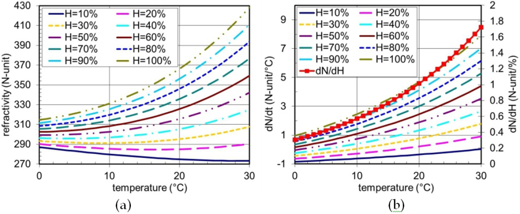
The radio refractivity dependence on temperature and relative humidity of air for pressure
The sensitivity of refractivity on temperature and relative humidity of air is shown in Fig. 1b. For t = 10º C (cca average near ground temperature in the Czech Republic), H = 70% (cca average near ground relative humidity) and p = 1000 hPa, the sensitivities are dN/dt = 1.43 N-unit/ºC, dN/dH = 0.57 N-unit/% and dN/dp = 0.27 N-unit/hPa. The refractivity variation is usually most significantly influenced by the changes of relative humidity as a water vapour content often changes rapidly (both in space and time) and it is least sensitive to pressure variation. However a decrease in pressure with altitude is mainly responsible for a standard vertical gradient of the atmospheric refractivity.
During standard atmospheric conditions, the temperature and pressure are decreasing with the height above the ground with lapse rates of about 6º C/km and 125 hPa/km (near ground gradients). Assuming that relative humidity is approximately constant with height, a standard value of the lapse rate of refractivity with a height h can be obtained using pressure and temperature sensitivities and their standard lapse rates. Such an estimated standard vertical gradient of refractivity is about dN/dh ≈ -42 N-units/km. It will be seen that such value is very close to the observed long term median of the vertical gradient of refractivity.
4.路徑剖面圖 (Path Profile)
地球表面高低起伏不同有平原 高山 建築物 湖泊 森林等分布 為了了解電波傳播的路線 常用K=4/3 的路徑剖面圖。


ESP32 遠端感應控制系統 目前的架構設計(結合了 ESP32、RFID、MQTT、Node-RED 與 Telegram 遠端雙向控制 ),這個系統的核心價值在於 即時感應、雲端中繼、智慧自動化與即時通訊回報 。 整個架構透過無線網路(Wi-Fi),將現場的硬體感測端、雲端訊...


