C語言 例題5-5.c 使用 二階Runge-Kutta 與 四階Runge-Kutta 解 ODE y'= -y + t^2 + 1 , 0<=t<=1 , y(0)=1 , 真實解 W(t)= -2e^(-t) + t ^2 - 2t + 3

C語言 例題5-5.c 使用 二階Runge-Kutta  與 四階Runge-Kutta 解 ODE y'= -y + t^2 + 1 , 0<=t<=1 , y(0)=1 , 真實解　W(t)= -2e^(-t) + t ^2 - 2t + 3

The most widely known member of the Runge–Kutta family is generally referred to as "RK4", the "classical Runge–Kutta method" or simply as "the Runge–Kutta method".

Let an initial value problem be specified as follows:

${\displaystyle {\dot {y}}=f(t,y),\quad y(t_{0})=y_{0}.}$

Here ${\displaystyle y}$ is an unknown function (scalar or vector) of time ${\displaystyle t}$, which we would like to approximate; we are told that ${\displaystyle {\dot {y}}}$, the rate at which ${\displaystyle y}$ changes, is a function of ${\displaystyle t}$ and of ${\displaystyle y}$ itself. At the initial time ${\displaystyle t_{0}}$ the corresponding ${\displaystyle y}$ value is ${\displaystyle y_{0}}$. The function ${\displaystyle f}$ and the data ${\displaystyle t_{0}}$, ${\displaystyle y_{0}}$ are given.

Now pick a step-size h > 0 and define

${\displaystyle {\begin{aligned}y_{n+1}&=y_{n}+{\tfrac {1}{6}}\left(k_{1}+2k_{2}+2k_{3}+k_{4}\right),\\t_{n+1}&=t_{n}+h\\\end{aligned}}}$

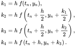
for n = 0, 1, 2, 3, ..., using^[2]

${\displaystyle {\begin{aligned}k_{1}&=h\ f(t_{n},y_{n}),\\k_{2}&=h\ f\left(t_{n}+{\frac {h}{2}},y_{n}+{\frac {k_{1}}{2}}\right),\\k_{3}&=h\ f\left(t_{n}+{\frac {h}{2}},y_{n}+{\frac {k_{2}}{2}}\right),\\k_{4}&=h\ f\left(t_{n}+h,y_{n}+k_{3}\right).\end{aligned}}}$

Lower step size means more accuracy.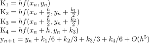

The formula basically computes next value yn+1 using current yn plus weighted average of four increments.

• k1 is the increment based on the slope at the beginning of the interval, using y
• k2 is the increment based on the slope at the midpoint of the interval, using y + hk1/2.
• k3 is again the increment based on the slope at the midpoint, using using y + hk2/2.
• k4 is the increment based on the slope at the end of the interval, using y + hk3.

/* ex5-5.c Second Order Runge-Kutta Method is used

 * for solving Ordinary Differential Equation of

 * y'=f(y,t) with initial condition of y(t0)=y0.

 */

#include <stdio.h>

#include <math.h>

#define F(y,t)   (-y+t*t+1)

#define W(t)     (-2*(1.0/exp(t))+pow(t,2)-2*t+3)

void main()

{

    int i,n=100;

    double h,a=0.0,b=1.0,t0,t,y0=1.0,y,k1,k2,k3,k4;

    h=(b-a)/n;

    y=y0;

    t0=a;

    t=t0;

    printf("t      y(t)       w(t)       error\n");

    printf("=====================================\n");

    printf("%.2lf %10.7lf %10.7lf %10.7lf\n\n",t,y,W(t),fabs(y-W(t)));

    for(i=1;i<=n;i++)

    {

        k1=h*F(y,t);

        k2=h*F((y+k1),(t+h));

        y=y+0.5*(k1+k2);

        t=t+h;

        if (i%10==0)

        {

            printf("k1=%.3lf , k2=%0.3lf\n",k1,k2);

            printf("%.2lf %10.7lf %10.7lf %10.7lf\n\n",t,y,W(t),fabs(y-W(t)));

        }    

    }

   

    h=(b-a)/n;

    y=y0;

    t0=a;

    t=t0;

    printf("t      y(t)       w(t)      error\n");

    printf("=====================================\n");

    printf("%.2lf %10.7lf %10.7lf %10.7lf\n\n" ,t,y,W(t),fabs(y-W(t)));

    for(i=1;i<=n;i++)

    {

        k1=h*F(y,t);

        k2=h*F((y+k1/2.0),(t+h/2.0));

        k3=h*F((y+k2/2.0),(t+h/2.0));

        k4=h*F((y+k3),(t+h));

        y=y+(k1+2*k2+2*k3+k4)/6.0;

        t=a+i*h;

        if(i%10==0)

        {

            printf("k1=%.3lf , k2=%0.3lf , k3=%0.3lf , k4=%0.3lf\n",k1,k2,k3,k4);

            printf("%.2lf %10.7lf %10.7lf %10.7lf\n\n",t,y,W(t),fabs(y-W(t)));

        }    

    }  

   return;

}

輸出畫面

t      y(t)       w(t)       error

=====================================

0.00  1.0000000  1.0000000  0.0000000

k1=0.000 , k2=0.000

0.10  1.0003269  1.0003252  0.0000017

k1=0.000 , k2=0.000

0.20  1.0025421  1.0025385  0.0000036

k1=0.001 , k2=0.001

0.30  1.0083691  1.0083636  0.0000056

k1=0.001 , k2=0.001

0.40  1.0193675  1.0193599  0.0000076

k1=0.002 , k2=0.002

0.50  1.0369483  1.0369387  0.0000096

k1=0.003 , k2=0.003

0.60  1.0623883  1.0623767  0.0000116

k1=0.004 , k2=0.004

0.70  1.0968430  1.0968294  0.0000136

k1=0.005 , k2=0.005

0.80  1.1413577  1.1413421  0.0000156

k1=0.006 , k2=0.006

0.90  1.1968782  1.1968607  0.0000175

k1=0.007 , k2=0.007

1.00  1.2642605  1.2642411  0.0000194

t      y(t)       w(t)      error

=====================================

0.00  1.0000000  1.0000000  0.0000000

k1=0.000 , k2=0.000 , k3=0.000 , k4=0.000

0.10  1.0003252  1.0003252  0.0000000

k1=0.000 , k2=0.000 , k3=0.000 , k4=0.000

0.20  1.0025385  1.0025385  0.0000000

k1=0.001 , k2=0.001 , k3=0.001 , k4=0.001

0.30  1.0083636  1.0083636  0.0000000

k1=0.001 , k2=0.001 , k3=0.001 , k4=0.001

0.40  1.0193599  1.0193599  0.0000000

k1=0.002 , k2=0.002 , k3=0.002 , k4=0.002

0.50  1.0369387  1.0369387  0.0000000

k1=0.003 , k2=0.003 , k3=0.003 , k4=0.003

0.60  1.0623767  1.0623767  0.0000000

k1=0.004 , k2=0.004 , k3=0.004 , k4=0.004

0.70  1.0968294  1.0968294  0.0000000

k1=0.005 , k2=0.005 , k3=0.005 , k4=0.005

0.80  1.1413421  1.1413421  0.0000000

k1=0.006 , k2=0.006 , k3=0.006 , k4=0.006

0.90  1.1968607  1.1968607  0.0000000

k1=0.007 , k2=0.007 , k3=0.007 , k4=0.007

1.00  1.2642411  1.2642411  0.0000000